Java Implement the Ann to Read Mnist
How to Develop a CNN for MNIST Handwritten Digit Classification
Last Updated on November fourteen, 2021
How to Develop a Convolutional Neural Network From Scratch for MNIST Handwritten Digit Classification.
The MNIST handwritten digit classification problem is a standard dataset used in calculator vision and deep learning.
Although the dataset is effectively solved, it can be used as the basis for learning and practicing how to develop, evaluate, and use convolutional deep learning neural networks for epitome classification from scratch. This includes how to develop a robust examination harness for estimating the functioning of the model, how to explore improvements to the model, and how to save the model and later load it to make predictions on new data.
In this tutorial, you volition discover how to develop a convolutional neural network for handwritten digit classification from scratch.
After completing this tutorial, y'all will know:
- How to develop a test harness to develop a robust evaluation of a model and constitute a baseline of performance for a classification task.
- How to explore extensions to a baseline model to improve learning and model capacity.
- How to develop a finalized model, evaluate the performance of the last model, and use it to make predictions on new images.
Kick-start your project with my new book Deep Learning for Computer Vision, including step-by-pace tutorials and the Python source lawmaking files for all examples.
Let'due south go started.
- Updated December/2019: Updated examples for TensorFlow 2.0 and Keras ii.three.
- Updated Jan/2020: Fixed a bug where models were defined outside the cantankerous-validation loop.
- Updated Nov/2021: Updated to use Tensorflow two.6
How to Develop a Convolutional Neural Network From Scratch for MNIST Handwritten Digit Classification
Photo past Richard Allaway, some rights reserved.
Tutorial Overview
This tutorial is divided into five parts; they are:
- MNIST Handwritten Digit Classification Dataset
- Model Evaluation Methodology
- How to Develop a Baseline Model
- How to Develop an Improved Model
- How to Finalize the Model and Brand Predictions
Desire Results with Deep Learning for Calculator Vision?
Accept my free vii-day email crash course at present (with sample code).
Click to sign-up and also get a free PDF Ebook version of the form.
Evolution Environment
This tutorial assumes that you are using standalone Keras running on top of TensorFlow with Python iii. If you demand assist setting up your development surround see this tutorial:
- How to Setup Your Python Environment for Automobile Learning with Anaconda
MNIST Handwritten Digit Nomenclature Dataset
The MNIST dataset is an acronym that stands for the Modified National Institute of Standards and Technology dataset.
It is a dataset of 60,000 small square 28×28 pixel grayscale images of handwritten single digits betwixt 0 and 9.
The task is to classify a given image of a handwritten digit into one of 10 classes representing integer values from 0 to 9, inclusively.
It is a widely used and deeply understood dataset and, for the nearly part, is "solved." Top-performing models are deep learning convolutional neural networks that achieve a classification accuracy of above 99%, with an mistake charge per unit between 0.4 %and 0.ii% on the hold out test dataset.
The example below loads the MNIST dataset using the Keras API and creates a plot of the start nine images in the training dataset.
| # instance of loading the mnist dataset from tensorflow . keras . datasets import mnist from matplotlib import pyplot as plt # load dataset ( trainX , trainy ) , ( testX , testy ) = mnist . load_data ( ) # summarize loaded dataset print ( 'Train: X=%s, y=%s' % ( trainX . shape , trainy . shape ) ) print ( 'Test: Ten=%due south, y=%s' % ( testX . shape , testy . shape ) ) # plot commencement few images for i in range ( 9 ) : # define subplot plt . subplot ( 330 + one + i ) # plot raw pixel data plt . imshow ( trainX [ i ] , cmap = plt . get_cmap ( 'gray' ) ) # show the figure plt . show ( ) |
Running the example loads the MNIST railroad train and exam dataset and prints their shape.
We can run across that there are 60,000 examples in the training dataset and 10,000 in the examination dataset and that images are indeed square with 28×28 pixels.
| Train: X=(60000, 28, 28), y=(60000,) Test: X=(10000, 28, 28), y=(10000,) |
A plot of the starting time ix images in the dataset is also created showing the natural handwritten nature of the images to be classified.
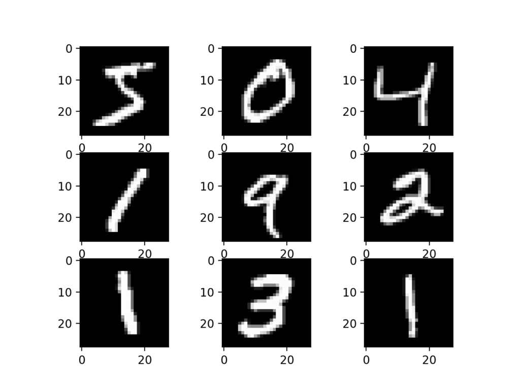
Plot of a Subset of Images From the MNIST Dataset
Model Evaluation Methodology
Although the MNIST dataset is finer solved, it can exist a useful starting point for developing and practicing a methodology for solving image nomenclature tasks using convolutional neural networks.
Instead of reviewing the literature on well-performing models on the dataset, we can develop a new model from scratch.
The dataset already has a well-defined train and exam dataset that we tin use.
In guild to judge the performance of a model for a given training run, we can farther split up the preparation prepare into a railroad train and validation dataset. Performance on the train and validation dataset over each run can then exist plotted to provide learning curves and insight into how well a model is learning the problem.
The Keras API supports this by specifying the "validation_data" argument to the model.fit() function when training the model, that will, in turn, return an object that describes model functioning for the chosen loss and metrics on each grooming epoch.
| # tape model functioning on a validation dataset during training history = model . fit ( . . . , validation_data = ( valX , valY ) ) |
In order to approximate the performance of a model on the problem in full general, we can use grand-fold cantankerous-validation, perhaps five-fold cantankerous-validation. This volition give some account of the models variance with both respect to differences in the training and test datasets, and in terms of the stochastic nature of the learning algorithm. The performance of a model tin be taken equally the hateful performance beyond k-folds, given the standard deviation, that could be used to gauge a confidence interval if desired.
We can use the KFold form from the scikit-learn API to implement the k-fold cross-validation evaluation of a given neural network model. In that location are many ways to achieve this, although we tin can choose a flexible approach where the KFold class is only used to specify the row indexes used for each spit.
| # example of 1000-fold cv for a neural internet data = . . . # gear up cross validation kfold = KFold ( 5 , shuffle = Truthful , random_state = 1 ) # enumerate splits for train_ix , test_ix in kfold . split ( data ) : model = . . . . . . |
We volition hold back the actual test dataset and utilise it as an evaluation of our last model.
How to Develop a Baseline Model
The first step is to develop a baseline model.
This is critical as it both involves developing the infrastructure for the examination harness and then that any model we pattern tin be evaluated on the dataset, and it establishes a baseline in model performance on the problem, by which all improvements tin be compared.
The pattern of the exam harness is modular, and we can develop a separate function for each piece. This allows a given aspect of the test harness to be modified or inter-inverse, if we want, separately from the rest.
We can develop this exam harness with five key elements. They are the loading of the dataset, the training of the dataset, the definition of the model, the evaluation of the model, and the presentation of results.
Load Dataset
We know some things about the dataset.
For case, we know that the images are all pre-aligned (e.g. each image but contains a manus-drawn digit), that the images all have the same square size of 28×28 pixels, and that the images are grayscale.
Therefore, nosotros can load the images and reshape the information arrays to have a unmarried color channel.
| # load dataset ( trainX , trainY ) , ( testX , testY ) = mnist . load_data ( ) # reshape dataset to take a single channel trainX = trainX . reshape ( ( trainX . shape [ 0 ] , 28 , 28 , i ) ) testX = testX . reshape ( ( testX . shape [ 0 ] , 28 , 28 , 1 ) ) |
We besides know that at that place are x classes and that classes are represented as unique integers.
We can, therefore, apply a one hot encoding for the course chemical element of each sample, transforming the integer into a 10 element binary vector with a ane for the index of the grade value, and 0 values for all other classes. We can achieve this with the to_categorical() utility function.
| # one hot encode target values trainY = to_categorical ( trainY ) testY = to_categorical ( testY ) |
The load_dataset() role implements these behaviors and can be used to load the dataset.
| # load train and exam dataset def load_dataset ( ) : # load dataset ( trainX , trainY ) , ( testX , testY ) = mnist . load_data ( ) # reshape dataset to have a single channel trainX = trainX . reshape ( ( trainX . shape [ 0 ] , 28 , 28 , 1 ) ) testX = testX . reshape ( ( testX . shape [ 0 ] , 28 , 28 , 1 ) ) # one hot encode target values trainY = to_categorical ( trainY ) testY = to_categorical ( testY ) render trainX , trainY , testX , testY |
Prepare Pixel Information
We know that the pixel values for each image in the dataset are unsigned integers in the range between black and white, or 0 and 255.
Nosotros practise non know the best way to calibration the pixel values for modeling, merely we know that some scaling will be required.
A good starting point is to normalize the pixel values of grayscale images, eastward.one thousand. rescale them to the range [0,1]. This involves first converting the data blazon from unsigned integers to floats, and so dividing the pixel values by the maximum value.
| # catechumen from integers to floats train_norm = train . astype ( 'float32' ) test_norm = test . astype ( 'float32' ) # normalize to range 0-1 train_norm = train_norm / 255.0 test_norm = test_norm / 255.0 |
The prep_pixels() function below implements these behaviors and is provided with the pixel values for both the train and test datasets that volition need to be scaled.
| # calibration pixels def prep_pixels ( train , examination ) : # catechumen from integers to floats train_norm = railroad train . astype ( 'float32' ) test_norm = test . astype ( 'float32' ) # normalize to range 0-i train_norm = train_norm / 255.0 test_norm = test_norm / 255.0 # return normalized images render train_norm , test_norm |
This office must exist called to prepare the pixel values prior to any modeling.
Define Model
Next, we need to define a baseline convolutional neural network model for the problem.
The model has ii main aspects: the feature extraction front finish comprised of convolutional and pooling layers, and the classifier backend that will make a prediction.
For the convolutional front-stop, we tin can start with a unmarried convolutional layer with a pocket-size filter size (3,iii) and a modest number of filters (32) followed by a max pooling layer. The filter maps can then be flattened to provide features to the classifier.
Given that the problem is a multi-class classification task, nosotros know that we will require an output layer with 10 nodes in order to predict the probability distribution of an image belonging to each of the 10 classes. This will also crave the utilize of a softmax activation function. Betwixt the characteristic extractor and the output layer, we can add together a dense layer to interpret the features, in this instance with 100 nodes.
All layers will use the ReLU activation function and the He weight initialization scheme, both best practices.
We will use a conservative configuration for the stochastic gradient descent optimizer with a learning charge per unit of 0.01 and a momentum of 0.9. The categorical cross-entropy loss function will be optimized, suitable for multi-class nomenclature, and we will monitor the classification accurateness metric, which is appropriate given we take the same number of examples in each of the 10 classes.
The define_model() role below will ascertain and return this model.
| # ascertain cnn model def define_model ( ) : model = Sequential ( ) model . add ( Conv2D ( 32 , ( 3 , iii ) , activation = 'relu' , kernel_initializer = 'he_uniform' , input_shape = ( 28 , 28 , 1 ) ) ) model . add together ( MaxPooling2D ( ( 2 , 2 ) ) ) model . add ( Flatten ( ) ) model . add ( Dense ( 100 , activation = 'relu' , kernel_initializer = 'he_uniform' ) ) model . add ( Dense ( 10 , activation = 'softmax' ) ) # compile model opt = SGD ( learning_rate = 0.01 , momentum = 0.ix ) model . compile ( optimizer = opt , loss = 'categorical_crossentropy' , metrics = [ 'accuracy' ] ) return model |
Evaluate Model
Afterward the model is divers, we need to evaluate it.
The model will exist evaluated using five-fold cross-validation. The value of one thousand=v was chosen to provide a baseline for both repeated evaluation and to not be and then large every bit to require a long running fourth dimension. Each exam set up will exist twenty% of the training dataset, or almost 12,000 examples, close to the size of the actual test set for this problem.
The training dataset is shuffled prior to being split, and the sample shuffling is performed each fourth dimension, and so that any model we evaluate volition have the same railroad train and exam datasets in each fold, providing an apples-to-apples comparison betwixt models.
We will train the baseline model for a modest 10 preparation epochs with a default batch size of 32 examples. The examination set for each fold will be used to evaluate the model both during each epoch of the grooming run, so that we can after create learning curves, and at the end of the run, so that we can estimate the performance of the model. As such, we will go along track of the resulting history from each run, as well as the nomenclature accurateness of the fold.
The evaluate_model() office below implements these behaviors, taking the training dataset equally arguments and returning a list of accurateness scores and preparation histories that can be afterwards summarized.
| 1 two 3 iv 5 6 seven 8 nine ten xi 12 13 14 fifteen 16 17 eighteen 19 20 | # evaluate a model using g-fold cantankerous-validation def evaluate_model ( dataX , dataY , n_folds = 5 ) : scores , histories = list ( ) , list ( ) # gear up cross validation kfold = KFold ( n_folds , shuffle = True , random_state = one ) # enumerate splits for train_ix , test_ix in kfold . split ( dataX ) : # define model model = define_model ( ) # select rows for train and exam trainX , trainY , testX , testY = dataX [ train_ix ] , dataY [ train_ix ] , dataX [ test_ix ] , dataY [ test_ix ] # fit model history = model . fit ( trainX , trainY , epochs = x , batch_size = 32 , validation_data = ( testX , testY ) , verbose = 0 ) # evaluate model _ , acc = model . evaluate ( testX , testY , verbose = 0 ) print ( '> %.3f' % ( acc * 100.0 ) ) # stores scores scores . append ( acc ) histories . append ( history ) return scores , histories |
Present Results
Once the model has been evaluated, we tin nowadays the results.
In that location are two key aspects to present: the diagnostics of the learning beliefs of the model during training and the interpretation of the model operation. These can exist implemented using separate functions.
Commencement, the diagnostics involve creating a line plot showing model functioning on the train and examination set during each fold of the g-fold cross-validation. These plots are valuable for getting an idea of whether a model is overfitting, underfitting, or has a skillful fit for the dataset.
We will create a single figure with two subplots, ane for loss and one for accuracy. Blueish lines volition indicate model performance on the training dataset and orange lines will bespeak performance on the hold out exam dataset. The summarize_diagnostics() part below creates and shows this plot given the nerveless grooming histories.
| # plot diagnostic learning curves def summarize_diagnostics ( histories ) : for i in range ( len ( histories ) ) : # plot loss plt . subplot ( ii , 1 , i ) plt . title ( 'Cross Entropy Loss' ) plt . plot ( histories [ i ] . history [ 'loss' ] , color = 'blueish' , label = 'train' ) plt . plot ( histories [ i ] . history [ 'val_loss' ] , colour = 'orange' , label = 'test' ) # plot accuracy plt . subplot ( 2 , 1 , ii ) plt . title ( 'Classification Accuracy' ) plt . plot ( histories [ i ] . history [ 'accurateness' ] , color = 'blueish' , characterization = 'railroad train' ) plt . plot ( histories [ i ] . history [ 'val_accuracy' ] , colour = 'orange' , label = 'test' ) plt . show ( ) |
Side by side, the classification accurateness scores collected during each fold can be summarized by computing the hateful and standard deviation. This provides an approximate of the boilerplate expected performance of the model trained on this dataset, with an estimate of the boilerplate variance in the hateful. We will also summarize the distribution of scores past creating and showing a box and whisker plot.
The summarize_performance() part below implements this for a given list of scores collected during model evaluation.
| # summarize model operation def summarize_performance ( scores ) : # impress summary print ( 'Accuracy: mean=%.3f std=%.3f, north=%d' % ( mean ( scores ) * 100 , std ( scores ) * 100 , len ( scores ) ) ) # box and whisker plots of results plt . boxplot ( scores ) plt . bear witness ( ) |
Complete Case
We need a function that will drive the exam harness.
This involves calling all of the define functions.
| # run the test harness for evaluating a model def run_test_harness ( ) : # load dataset trainX , trainY , testX , testY = load_dataset ( ) # prepare pixel data trainX , testX = prep_pixels ( trainX , testX ) # evaluate model scores , histories = evaluate_model ( trainX , trainY ) # learning curves summarize_diagnostics ( histories ) # summarize estimated performance summarize_performance ( scores ) |
We now have everything we need; the complete code instance for a baseline convolutional neural network model on the MNIST dataset is listed below.
| 1 2 iii iv 5 six 7 viii nine x 11 12 13 14 fifteen 16 17 18 19 xx 21 22 23 24 25 26 27 28 29 30 31 32 33 34 35 36 37 38 39 40 41 42 43 44 45 46 47 48 49 50 51 52 53 54 55 56 57 58 59 60 61 62 63 64 65 66 67 68 69 70 71 72 73 74 75 76 77 78 79 80 81 82 83 84 85 86 87 88 89 xc 91 92 93 94 95 96 97 98 99 100 101 102 103 104 105 106 107 108 109 | # baseline cnn model for mnist from numpy import mean from numpy import std from matplotlib import pyplot as plt from sklearn . model_selection import KFold from tensorflow . keras . datasets import mnist from tensorflow . keras . utils import to_categorical from tensorflow . keras . models import Sequential from tensorflow . keras . layers import Conv2D from tensorflow . keras . layers import MaxPooling2D from tensorflow . keras . layers import Dumbo from tensorflow . keras . layers import Flatten from tensorflow . keras . optimizers import SGD # load railroad train and exam dataset def load_dataset ( ) : # load dataset ( trainX , trainY ) , ( testX , testY ) = mnist . load_data ( ) # reshape dataset to have a single channel trainX = trainX . reshape ( ( trainX . shape [ 0 ] , 28 , 28 , 1 ) ) testX = testX . reshape ( ( testX . shape [ 0 ] , 28 , 28 , 1 ) ) # one hot encode target values trainY = to_categorical ( trainY ) testY = to_categorical ( testY ) return trainX , trainY , testX , testY # calibration pixels def prep_pixels ( train , test ) : # convert from integers to floats train_norm = train . astype ( 'float32' ) test_norm = test . astype ( 'float32' ) # normalize to range 0-1 train_norm = train_norm / 255.0 test_norm = test_norm / 255.0 # return normalized images return train_norm , test _norm # define cnn model def define_model ( ) : model = Sequential ( ) model . add ( Conv2D ( 32 , ( 3 , three ) , activation = 'relu' , kernel_initializer = 'he_uniform' , input_shape = ( 28 , 28 , ane ) ) ) model . add ( MaxPooling2D ( ( 2 , 2 ) ) ) model . add together ( Flatten ( ) ) model . add together ( Dense ( 100 , activation = 'relu' , kernel_initializer = 'he_uniform' ) ) model . add ( Dense ( 10 , activation = 'softmax' ) ) # compile model opt = SGD ( learning_rate = 0.01 , momentum = 0.9 ) model . compile ( optimizer = opt , loss = 'categorical_crossentropy' , metrics = [ 'accuracy' ] ) return model # evaluate a model using 1000-fold cross-validation def evaluate_model ( dataX , dataY , n_folds = 5 ) : scores , histories = list ( ) , listing ( ) # prepare cross validation kfold = KFold ( n_folds , shuffle = True , random_state = i ) # enumerate splits for train_ix , test_ix in kfold . split ( dataX ) : # define model model = define_model ( ) # select rows for train and examination trainX , trainY , testX , testY = dataX [ train_ix ] , dataY [ train_ix ] , dataX [ test_ix ] , dataY [ test_ix ] # fit model history = model . fit ( trainX , trainY , epochs = 10 , batch_size = 32 , validation_data = ( testX , testY ) , verbose = 0 ) # evaluate model _ , acc = model . evaluate ( testX , testY , verbose = 0 ) impress ( '> %.3f' % ( acc * 100.0 ) ) # stores scores scores . append ( acc ) histories . append ( history ) return scores , histories # plot diagnostic learning curves def summarize_diagnostics ( histories ) : for i in range ( len ( histories ) ) : # plot loss plt . subplot ( 2 , 1 , 1 ) plt . championship ( 'Cross Entropy Loss' ) plt . plot ( histories [ i ] . history [ 'loss' ] , color = 'bluish' , characterization = 'train' ) plt . plot ( histories [ i ] . history [ 'val_loss' ] , colour = 'orangish' , label = 'test' ) # plot accuracy plt . subplot ( 2 , 1 , two ) plt . championship ( 'Classification Accurateness' ) plt . plot ( histories [ i ] . history [ 'accuracy' ] , colour = 'blue' , characterization = 'train' ) plt . plot ( histories [ i ] . history [ 'val_accuracy' ] , colour = 'orangish' , label = 'test' ) plt . show ( ) # summarize model performance def summarize_performance ( scores ) : # print summary impress ( 'Accuracy: mean=%.3f std=%.3f, n=%d' % ( mean ( scores ) * 100 , std ( scores ) * 100 , len ( scores ) ) ) # box and whisker plots of results plt . boxplot ( scores ) plt . bear witness ( ) # run the test harness for evaluating a model def run_test_harness ( ) : # load dataset trainX , trainY , testX , testY = load_dataset ( ) # prepare pixel data trainX , testX = prep_pixels ( trainX , testX ) # evaluate model scores , histories = evaluate_model ( trainX , trainY ) # learning curves summarize_diagnostics ( histories ) # summarize estimated performance summarize_performance ( scores ) # entry bespeak, run the exam harness run_test_harness ( ) |
Running the example prints the classification accuracy for each fold of the cantankerous-validation procedure. This is helpful to get an thought that the model evaluation is progressing.
Note: Your results may vary given the stochastic nature of the algorithm or evaluation procedure, or differences in numerical precision. Consider running the example a few times and compare the average upshot.
We can see two cases where the model achieves perfect skill and ane case where it accomplished lower than 98% accuracy. These are good results.
| > 98.550 > 98.600 > 98.642 > 98.850 > 98.742 |
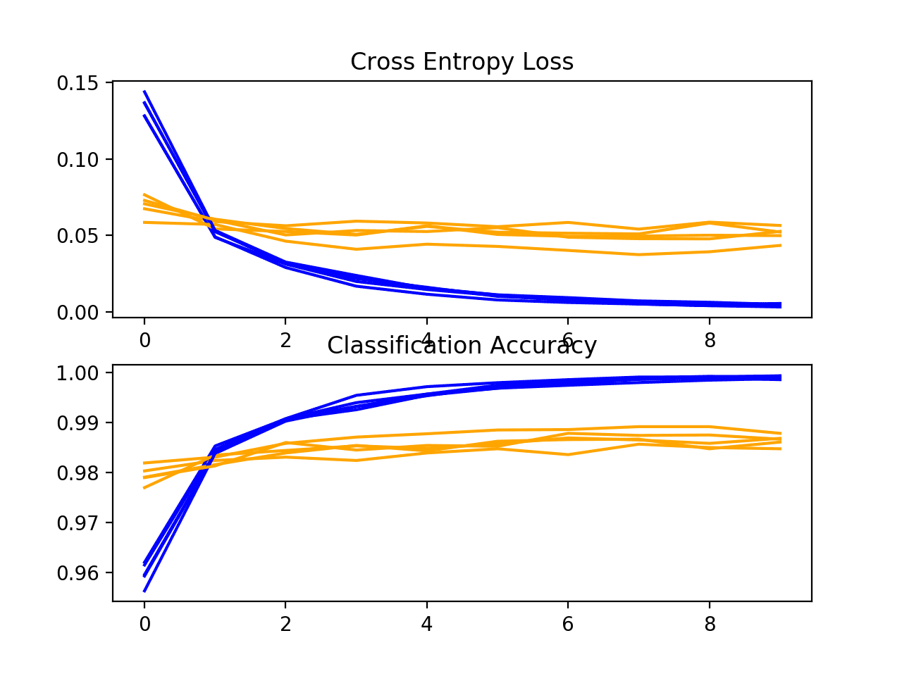
Next, a diagnostic plot is shown, giving insight into the learning behavior of the model across each fold.
In this instance, we tin run across that the model generally achieves a good fit, with train and examination learning curves converging. In that location is no obvious sign of over- or underfitting.
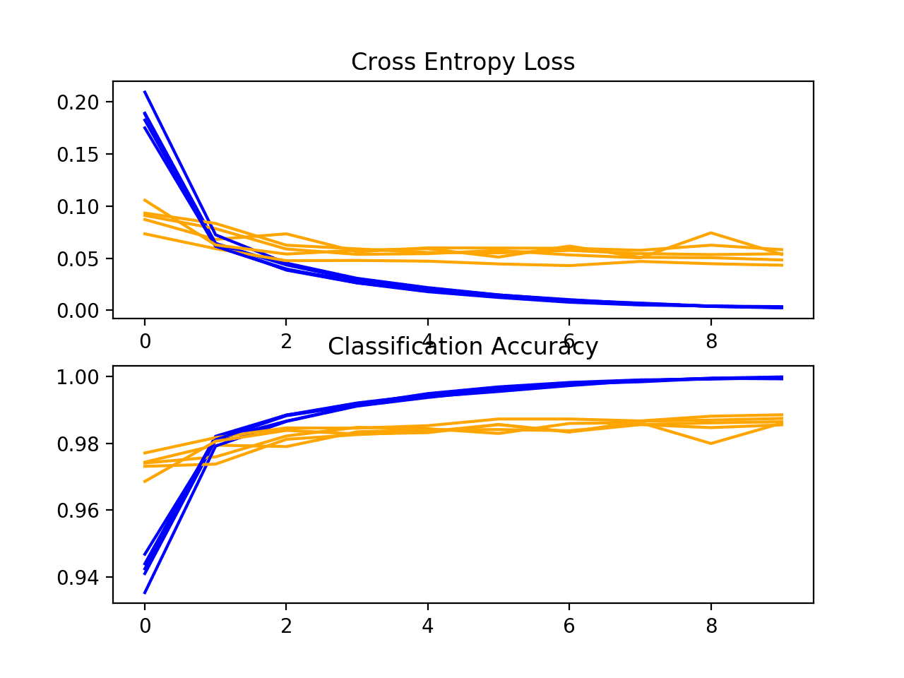
Loss and Accuracy Learning Curves for the Baseline Model During k-Fold Cantankerous-Validation
Next, a summary of the model performance is calculated.
Nosotros tin meet in this instance, the model has an estimated skill of about 98.half-dozen%, which is reasonable.
| Accuracy: hateful=98.677 std=0.107, northward=5 |
Finally, a box and whisker plot is created to summarize the distribution of accuracy scores.
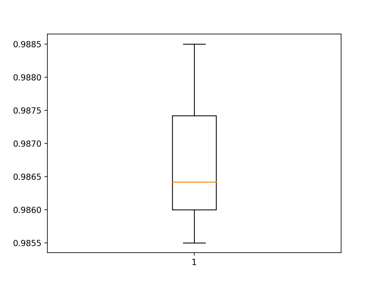
Box and Whisker Plot of Accuracy Scores for the Baseline Model Evaluated Using thou-Fold Cantankerous-Validation
We now have a robust test harness and a well-performing baseline model.
How to Develop an Improved Model
At that place are many ways that we might explore improvements to the baseline model.
We will look at areas of model configuration that often consequence in an improvement, so-called low-hanging fruit. The first is a change to the learning algorithm, and the second is an increase in the depth of the model.
Comeback to Learning
At that place are many aspects of the learning algorithm that can be explored for improvement.
Perhaps the point of biggest leverage is the learning charge per unit, such every bit evaluating the touch that smaller or larger values of the learning rate may take, as well as schedules that alter the learning rate during training.
Another arroyo that can rapidly accelerate the learning of a model and can effect in large performance improvements is batch normalization. We will evaluate the outcome that batch normalization has on our baseline model.
Batch normalization tin can be used after convolutional and fully continued layers. It has the consequence of changing the distribution of the output of the layer, specifically by standardizing the outputs. This has the event of stabilizing and accelerating the learning procedure.
Nosotros can update the model definition to use batch normalization after the activation office for the convolutional and dense layers of our baseline model. The updated version of define_model() function with batch normalization is listed beneath.
| # define cnn model def define_model ( ) : model = Sequential ( ) model . add together ( Conv2D ( 32 , ( 3 , three ) , activation = 'relu' , kernel_initializer = 'he_uniform' , input_shape = ( 28 , 28 , 1 ) ) ) model . add together ( BatchNormalization ( ) ) model . add together ( MaxPooling2D ( ( 2 , ii ) ) ) model . add ( Flatten ( ) ) model . add ( Dumbo ( 100 , activation = 'relu' , kernel_initializer = 'he_uniform' ) ) model . add together ( BatchNormalization ( ) ) model . add ( Dense ( x , activation = 'softmax' ) ) # compile model opt = SGD ( learning_rate = 0.01 , momentum = 0.9 ) model . compile ( optimizer = opt , loss = 'categorical_crossentropy' , metrics = [ 'accuracy' ] ) return model |
The complete code list with this change is provided beneath.
| i 2 iii four 5 half dozen vii 8 9 10 xi 12 13 xiv 15 16 17 18 19 20 21 22 23 24 25 26 27 28 29 30 31 32 33 34 35 36 37 38 39 40 41 42 43 44 45 46 47 48 49 50 51 52 53 54 55 56 57 58 59 threescore 61 62 63 64 65 66 67 68 69 70 71 72 73 74 75 76 77 78 79 lxxx 81 82 83 84 85 86 87 88 89 90 91 92 93 94 95 96 97 98 99 100 101 102 103 104 105 106 107 108 109 110 111 112 | # cnn model with batch normalization for mnist from numpy import mean from numpy import std from matplotlib import pyplot as plt from sklearn . model_selection import KFold from tensorflow . keras . datasets import mnist from tensorflow . keras . utils import to_categorical from tensorflow . keras . models import Sequential from tensorflow . keras . layers import Conv2D from tensorflow . keras . layers import MaxPooling2D from tensorflow . keras . layers import Dense from tensorflow . keras . layers import Flatten from tensorflow . keras . optimizers import SGD from tensorflow . keras . layers import BatchNormalization # load train and test dataset def load_dataset ( ) : # load dataset ( trainX , trainY ) , ( testX , testY ) = mnist . load_data ( ) # reshape dataset to have a single channel trainX = trainX . reshape ( ( trainX . shape [ 0 ] , 28 , 28 , 1 ) ) testX = testX . reshape ( ( testX . shape [ 0 ] , 28 , 28 , i ) ) # one hot encode target values trainY = to_categorical ( trainY ) testY = to_categorical ( testY ) return trainX , trainY , testX , testY # calibration pixels def prep_pixels ( train , test ) : # catechumen from integers to floats train_norm = train . astype ( 'float32' ) test_norm = test . astype ( 'float32' ) # normalize to range 0-1 train_norm = train_norm / 255.0 test_norm = test_norm / 255.0 # return normalized images return train_norm , examination _norm # define cnn model def define_model ( ) : model = Sequential ( ) model . add ( Conv2D ( 32 , ( three , 3 ) , activation = 'relu' , kernel_initializer = 'he_uniform' , input_shape = ( 28 , 28 , 1 ) ) ) model . add ( BatchNormalization ( ) ) model . add ( MaxPooling2D ( ( two , ii ) ) ) model . add ( Flatten ( ) ) model . add ( Dumbo ( 100 , activation = 'relu' , kernel_initializer = 'he_uniform' ) ) model . add ( BatchNormalization ( ) ) model . add ( Dense ( 10 , activation = 'softmax' ) ) # compile model opt = SGD ( learning_rate = 0.01 , momentum = 0.9 ) model . compile ( optimizer = opt , loss = 'categorical_crossentropy' , metrics = [ 'accuracy' ] ) render model # evaluate a model using k-fold cross-validation def evaluate_model ( dataX , dataY , n_folds = 5 ) : scores , histories = list ( ) , list ( ) # prepare cross validation kfold = KFold ( n_folds , shuffle = True , random_state = 1 ) # enumerate splits for train_ix , test_ix in kfold . split ( dataX ) : # define model model = define_model ( ) # select rows for train and exam trainX , trainY , testX , testY = dataX [ train_ix ] , dataY [ train_ix ] , dataX [ test_ix ] , dataY [ test_ix ] # fit model history = model . fit ( trainX , trainY , epochs = x , batch_size = 32 , validation_data = ( testX , testY ) , verbose = 0 ) # evaluate model _ , acc = model . evaluate ( testX , testY , verbose = 0 ) print ( '> %.3f' % ( acc * 100.0 ) ) # stores scores scores . append ( acc ) histories . suspend ( history ) return scores , histories # plot diagnostic learning curves def summarize_diagnostics ( histories ) : for i in range ( len ( histories ) ) : # plot loss plt . subplot ( 2 , 1 , 1 ) plt . championship ( 'Cross Entropy Loss' ) plt . plot ( histories [ i ] . history [ 'loss' ] , color = 'blue' , label = 'train' ) plt . plot ( histories [ i ] . history [ 'val_loss' ] , colour = 'orange' , label = 'test' ) # plot accuracy plt . subplot ( 2 , one , 2 ) plt . title ( 'Classification Accuracy' ) plt . plot ( histories [ i ] . history [ 'accuracy' ] , colour = 'blueish' , characterization = 'railroad train' ) plt . plot ( histories [ i ] . history [ 'val_accuracy' ] , colour = 'orange' , characterization = 'exam' ) plt . show ( ) # summarize model performance def summarize_performance ( scores ) : # print summary print ( 'Accuracy: mean=%.3f std=%.3f, n=%d' % ( mean ( scores ) * 100 , std ( scores ) * 100 , len ( scores ) ) ) # box and whisker plots of results plt . boxplot ( scores ) plt . prove ( ) # run the test harness for evaluating a model def run_test_harness ( ) : # load dataset trainX , trainY , testX , testY = load_dataset ( ) # gear up pixel information trainX , testX = prep_pixels ( trainX , testX ) # evaluate model scores , histories = evaluate_model ( trainX , trainY ) # learning curves summarize_diagnostics ( histories ) # summarize estimated performance summarize_performance ( scores ) # entry point, run the examination harness run_test_harness ( ) |
Running the case once again reports model performance for each fold of the cross-validation procedure.
Note: Your results may vary given the stochastic nature of the algorithm or evaluation procedure, or differences in numerical precision. Consider running the instance a few times and compare the average outcome.
We can meet perhaps a pocket-size drop in model performance equally compared to the baseline across the cantankerous-validation folds.
| > 98.475 > 98.608 > 98.683 > 98.783 > 98.667 |
A plot of the learning curves is created, in this case showing that the speed of learning (comeback over epochs) does non announced to exist different from the baseline model.
The plots propose that batch normalization, at least as implemented in this case, does not offer any do good.
Loss and Accuracy Learning Curves for the BatchNormalization Model During chiliad-Fold Cantankerous-Validation
Next, the estimated performance of the model is presented, showing functioning with a slight decrease in the mean accurateness of the model: 98.643 every bit compared to 98.677 with the baseline model.
| Accurateness: mean=98.643 std=0.101, n=5 |

Box and Whisker Plot of Accuracy Scores for the BatchNormalization Model Evaluated Using grand-Fold Cross-Validation
Increase in Model Depth
There are many ways to change the model configuration in order to explore improvements over the baseline model.
Two mutual approaches involve changing the capacity of the feature extraction part of the model or irresolute the capacity or function of the classifier part of the model. Perhaps the point of biggest influence is a modify to the feature extractor.
We tin can increment the depth of the feature extractor part of the model, following a VGG-like blueprint of calculation more than convolutional and pooling layers with the aforementioned sized filter, while increasing the number of filters. In this example, we volition add a double convolutional layer with 64 filters each, followed past another max pooling layer.
The updated version of the define_model() function with this change is listed beneath.
| # define cnn model def define_model ( ) : model = Sequential ( ) model . add ( Conv2D ( 32 , ( 3 , 3 ) , activation = 'relu' , kernel_initializer = 'he_uniform' , input_shape = ( 28 , 28 , one ) ) ) model . add ( MaxPooling2D ( ( 2 , two ) ) ) model . add ( Conv2D ( 64 , ( 3 , 3 ) , activation = 'relu' , kernel_initializer = 'he_uniform' ) ) model . add ( Conv2D ( 64 , ( 3 , 3 ) , activation = 'relu' , kernel_initializer = 'he_uniform' ) ) model . add ( MaxPooling2D ( ( 2 , 2 ) ) ) model . add ( Flatten ( ) ) model . add ( Dense ( 100 , activation = 'relu' , kernel_initializer = 'he_uniform' ) ) model . add together ( Dumbo ( 10 , activation = 'softmax' ) ) # compile model opt = SGD ( learning_rate = 0.01 , momentum = 0.ix ) model . compile ( optimizer = opt , loss = 'categorical_crossentropy' , metrics = [ 'accuracy' ] ) render model |
For abyss, the entire code list, including this change, is provided below.
| 1 two 3 4 5 six 7 viii 9 10 xi 12 13 fourteen xv 16 17 18 xix 20 21 22 23 24 25 26 27 28 29 thirty 31 32 33 34 35 36 37 38 39 40 41 42 43 44 45 46 47 48 49 fifty 51 52 53 54 55 56 57 58 59 60 61 62 63 64 65 66 67 68 69 70 71 72 73 74 75 76 77 78 79 80 81 82 83 84 85 86 87 88 89 90 91 92 93 94 95 96 97 98 99 100 101 102 103 104 105 106 107 108 109 110 111 112 | # deeper cnn model for mnist from numpy import hateful from numpy import std from matplotlib import pyplot as plt from sklearn . model_selection import KFold from tensorflow . keras . datasets import mnist from tensorflow . keras . utils import to_categorical from tensorflow . keras . models import Sequential from tensorflow . keras . layers import Conv2D from tensorflow . keras . layers import MaxPooling2D from tensorflow . keras . layers import Dense from tensorflow . keras . layers import Flatten from tensorflow . keras . optimizers import SGD # load railroad train and test dataset def load_dataset ( ) : # load dataset ( trainX , trainY ) , ( testX , testY ) = mnist . load_data ( ) # reshape dataset to have a unmarried channel trainX = trainX . reshape ( ( trainX . shape [ 0 ] , 28 , 28 , i ) ) testX = testX . reshape ( ( testX . shape [ 0 ] , 28 , 28 , 1 ) ) # one hot encode target values trainY = to_categorical ( trainY ) testY = to_categorical ( testY ) return trainX , trainY , testX , testY # scale pixels def prep_pixels ( train , exam ) : # convert from integers to floats train_norm = train . astype ( 'float32' ) test_norm = test . astype ( 'float32' ) # normalize to range 0-1 train_norm = train_norm / 255.0 test_norm = test_norm / 255.0 # return normalized images return train_norm , examination _norm # ascertain cnn model def define_model ( ) : model = Sequential ( ) model . add ( Conv2D ( 32 , ( 3 , 3 ) , activation = 'relu' , kernel_initializer = 'he_uniform' , input_shape = ( 28 , 28 , ane ) ) ) model . add ( MaxPooling2D ( ( ii , ii ) ) ) model . add ( Conv2D ( 64 , ( three , three ) , activation = 'relu' , kernel_initializer = 'he_uniform' ) ) model . add ( Conv2D ( 64 , ( three , 3 ) , activation = 'relu' , kernel_initializer = 'he_uniform' ) ) model . add ( MaxPooling2D ( ( 2 , 2 ) ) ) model . add ( Flatten ( ) ) model . add ( Dumbo ( 100 , activation = 'relu' , kernel_initializer = 'he_uniform' ) ) model . add ( Dense ( 10 , activation = 'softmax' ) ) # compile model opt = SGD ( learning_rate = 0.01 , momentum = 0.9 ) model . compile ( optimizer = opt , loss = 'categorical_crossentropy' , metrics = [ 'accuracy' ] ) return model # evaluate a model using k-fold cross-validation def evaluate_model ( dataX , dataY , n_folds = 5 ) : scores , histories = list ( ) , list ( ) # prepare cross validation kfold = KFold ( n_folds , shuffle = True , random_state = 1 ) # enumerate splits for train_ix , test_ix in kfold . split ( dataX ) : # define model model = define_model ( ) # select rows for train and test trainX , trainY , testX , testY = dataX [ train_ix ] , dataY [ train_ix ] , dataX [ test_ix ] , dataY [ test_ix ] # fit model history = model . fit ( trainX , trainY , epochs = 10 , batch_size = 32 , validation_data = ( testX , testY ) , verbose = 0 ) # evaluate model _ , acc = model . evaluate ( testX , testY , verbose = 0 ) impress ( '> %.3f' % ( acc * 100.0 ) ) # stores scores scores . append ( acc ) histories . append ( history ) return scores , histories # plot diagnostic learning curves def summarize_diagnostics ( histories ) : for i in range ( len ( histories ) ) : # plot loss plt . subplot ( 2 , 1 , 1 ) plt . title ( 'Cantankerous Entropy Loss' ) plt . plot ( histories [ i ] . history [ 'loss' ] , color = 'blue' , label = 'railroad train' ) plt . plot ( histories [ i ] . history [ 'val_loss' ] , color = 'orange' , label = 'test' ) # plot accuracy plt . subplot ( two , 1 , 2 ) plt . championship ( 'Classification Accurateness' ) plt . plot ( histories [ i ] . history [ 'accuracy' ] , color = 'blue' , label = 'train' ) plt . plot ( histories [ i ] . history [ 'val_accuracy' ] , color = 'orange' , label = 'exam' ) plt . prove ( ) # summarize model functioning def summarize_performance ( scores ) : # print summary print ( 'Accuracy: mean=%.3f std=%.3f, n=%d' % ( mean ( scores ) * 100 , std ( scores ) * 100 , len ( scores ) ) ) # box and whisker plots of results plt . boxplot ( scores ) plt . prove ( ) # run the exam harness for evaluating a model def run_test_harness ( ) : # load dataset trainX , trainY , testX , testY = load_dataset ( ) # prepare pixel data trainX , testX = prep_pixels ( trainX , testX ) # evaluate model scores , histories = evaluate_model ( trainX , trainY ) # learning curves summarize_diagnostics ( histories ) # summarize estimated performance summarize_performance ( scores ) # entry bespeak, run the examination harness run_test_harness ( ) |
Running the example reports model performance for each fold of the cross-validation process.
Note: Your results may vary given the stochastic nature of the algorithm or evaluation procedure, or differences in numerical precision. Consider running the example a few times and compare the boilerplate outcome.
The per-fold scores may suggest some improvement over the baseline.
| > 99.058 > 99.042 > 98.883 > 99.192 > 99.133 |
A plot of the learning curves is created, in this case showing that the models however accept a good fit on the problem, with no articulate signs of overfitting. The plots may even suggest that further training epochs could exist helpful.
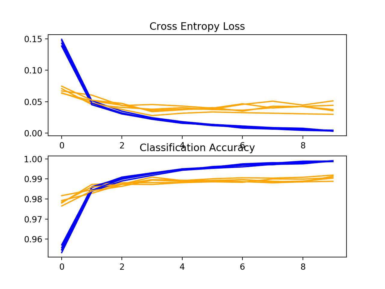
Loss and Accuracy Learning Curves for the Deeper Model During k-Fold Cross-Validation
Next, the estimated operation of the model is presented, showing a pocket-size comeback in performance as compared to the baseline from 98.677 to 99.062, with a small driblet in the standard departure too.
| Accuracy: mean=99.062 std=0.104, due north=five |
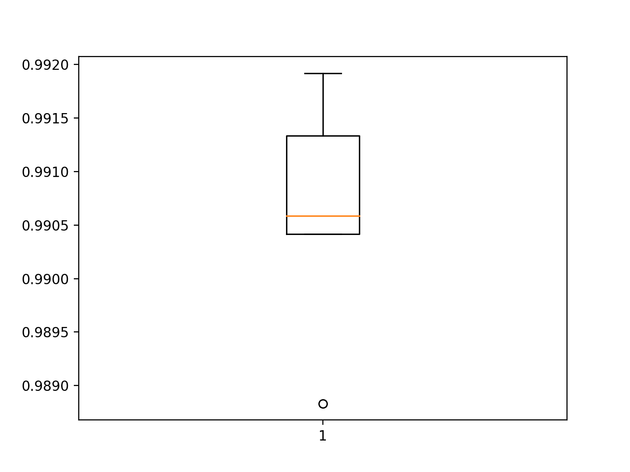
Box and Whisker Plot of Accuracy Scores for the Deeper Model Evaluated Using k-Fold Cross-Validation
How to Finalize the Model and Make Predictions
The process of model improvement may continue for as long as we have ideas and the fourth dimension and resources to test them out.
At some point, a final model configuration must be called and adopted. In this example, we will choose the deeper model as our final model.
First, we will finalize our model, but fitting a model on the unabridged training dataset and saving the model to file for afterward use. We will then load the model and evaluate its functioning on the hold out examination dataset to get an idea of how well the chosen model actually performs in practice. Finally, nosotros will use the saved model to brand a prediction on a single epitome.
Relieve Final Model
A final model is typically fit on all bachelor data, such as the combination of all railroad train and test dataset.
In this tutorial, nosotros are intentionally holding back a exam dataset then that we can estimate the performance of the final model, which can be a practiced thought in practice. Equally such, we will fit our model on the grooming dataset only.
| # fit model model . fit ( trainX , trainY , epochs = 10 , batch_size = 32 , verbose = 0 ) |
In one case fit, we can save the terminal model to an H5 file past calling the save() function on the model and pass in the called filename.
| # save model model . relieve ( 'final_model.h5' ) |
Note, saving and loading a Keras model requires that the h5py library is installed on your workstation.
The consummate example of plumbing fixtures the final deep model on the grooming dataset and saving it to file is listed below.
| 1 ii iii 4 5 half dozen 7 8 9 10 eleven 12 13 14 xv xvi 17 eighteen 19 twenty 21 22 23 24 25 26 27 28 29 30 31 32 33 34 35 36 37 38 39 40 41 42 43 44 45 46 47 48 49 fifty 51 52 53 54 55 56 57 58 59 60 61 62 63 64 | # relieve the final model to file from tensorflow . keras . datasets import mnist from tensorflow . keras . utils import to_categorical from tensorflow . keras . models import Sequential from tensorflow . keras . layers import Conv2D from tensorflow . keras . layers import MaxPooling2D from tensorflow . keras . layers import Dense from tensorflow . keras . layers import Flatten from tensorflow . keras . optimizers import SGD # load railroad train and exam dataset def load_dataset ( ) : # load dataset ( trainX , trainY ) , ( testX , testY ) = mnist . load_data ( ) # reshape dataset to have a unmarried aqueduct trainX = trainX . reshape ( ( trainX . shape [ 0 ] , 28 , 28 , 1 ) ) testX = testX . reshape ( ( testX . shape [ 0 ] , 28 , 28 , one ) ) # 1 hot encode target values trainY = to_categorical ( trainY ) testY = to_categorical ( testY ) render trainX , trainY , testX , testY # scale pixels def prep_pixels ( train , test ) : # convert from integers to floats train_norm = train . astype ( 'float32' ) test_norm = exam . astype ( 'float32' ) # normalize to range 0-i train_norm = train_norm / 255.0 test_norm = test_norm / 255.0 # render normalized images return train_norm , test _norm # define cnn model def define_model ( ) : model = Sequential ( ) model . add ( Conv2D ( 32 , ( 3 , 3 ) , activation = 'relu' , kernel_initializer = 'he_uniform' , input_shape = ( 28 , 28 , 1 ) ) ) model . add ( MaxPooling2D ( ( 2 , 2 ) ) ) model . add ( Conv2D ( 64 , ( 3 , three ) , activation = 'relu' , kernel_initializer = 'he_uniform' ) ) model . add ( Conv2D ( 64 , ( three , iii ) , activation = 'relu' , kernel_initializer = 'he_uniform' ) ) model . add together ( MaxPooling2D ( ( ii , 2 ) ) ) model . add together ( Flatten ( ) ) model . add ( Dumbo ( 100 , activation = 'relu' , kernel_initializer = 'he_uniform' ) ) model . add ( Dumbo ( x , activation = 'softmax' ) ) # compile model opt = SGD ( learning_rate = 0.01 , momentum = 0.9 ) model . compile ( optimizer = opt , loss = 'categorical_crossentropy' , metrics = [ 'accuracy' ] ) render model # run the examination harness for evaluating a model def run_test_harness ( ) : # load dataset trainX , trainY , testX , testY = load_dataset ( ) # prepare pixel data trainX , testX = prep_pixels ( trainX , testX ) # ascertain model model = define_model ( ) # fit model model . fit ( trainX , trainY , epochs = 10 , batch_size = 32 , verbose = 0 ) # save model model . save ( 'final_model.h5' ) # entry indicate, run the test harness run_test_harness ( ) |
After running this case, you volition at present have a ane.2-megabyte file with the name 'final_model.h5' in your current working directory.
Evaluate Final Model
We can at present load the final model and evaluate it on the concord out test dataset.
This is something we might do if nosotros were interested in presenting the performance of the chosen model to project stakeholders.
The model tin be loaded via the load_model() function.
The complete example of loading the saved model and evaluating it on the test dataset is listed below.
| 1 2 3 4 5 6 7 viii nine 10 eleven 12 xiii 14 15 sixteen 17 xviii 19 20 21 22 23 24 25 26 27 28 29 xxx 31 32 33 34 35 36 37 38 39 40 41 42 | # evaluate the deep model on the examination dataset from tensorflow . keras . datasets import mnist from tensorflow . keras . models import load_model from tensorflow . keras . utils import to _categorical # load train and examination dataset def load_dataset ( ) : # load dataset ( trainX , trainY ) , ( testX , testY ) = mnist . load_data ( ) # reshape dataset to take a unmarried aqueduct trainX = trainX . reshape ( ( trainX . shape [ 0 ] , 28 , 28 , ane ) ) testX = testX . reshape ( ( testX . shape [ 0 ] , 28 , 28 , 1 ) ) # one hot encode target values trainY = to_categorical ( trainY ) testY = to_categorical ( testY ) return trainX , trainY , testX , testY # scale pixels def prep_pixels ( train , examination ) : # convert from integers to floats train_norm = railroad train . astype ( 'float32' ) test_norm = exam . astype ( 'float32' ) # normalize to range 0-i train_norm = train_norm / 255.0 test_norm = test_norm / 255.0 # return normalized images return train_norm , exam _norm # run the test harness for evaluating a model def run_test_harness ( ) : # load dataset trainX , trainY , testX , testY = load_dataset ( ) # set up pixel data trainX , testX = prep_pixels ( trainX , testX ) # load model model = load_model ( 'final_model.h5' ) # evaluate model on exam dataset _ , acc = model . evaluate ( testX , testY , verbose = 0 ) print ( '> %.3f' % ( acc * 100.0 ) ) # entry bespeak, run the test harness run_test_harness ( ) |
Running the instance loads the saved model and evaluates the model on the hold out test dataset.
Note: Your results may vary given the stochastic nature of the algorithm or evaluation procedure, or differences in numerical precision. Consider running the example a few times and compare the boilerplate outcome.
The classification accuracy for the model on the test dataset is calculated and printed. In this case, we tin can see that the model accomplished an accuracy of 99.090%, or only less than 1%, which is non bad at all and reasonably shut to the estimated 99.753% with a standard deviation of near half a pct (e.thousand. 99% of scores).
Make Prediction
Nosotros tin can employ our saved model to make a prediction on new images.
The model assumes that new images are grayscale, that they have been aligned so that one image contains 1 centered handwritten digit, and that the size of the paradigm is foursquare with the size 28×28 pixels.
Below is an paradigm extracted from the MNIST test dataset. You can salve it in your electric current working directory with the filename 'sample_image.png'.

Sample Handwritten Digit
- Download the sample image (sample_image.png)
We will pretend this is an entirely new and unseen image, prepared in the required way, and see how we might utilize our saved model to predict the integer that the image represents (e.g. we look "7").
Get-go, nosotros can load the image, force information technology to exist in grayscale format, and strength the size to be 28×28 pixels. The loaded prototype can so be resized to have a single channel and represent a single sample in a dataset. The load_image() function implements this and volition return the loaded prototype ready for classification.
Importantly, the pixel values are prepared in the same way as the pixel values were prepared for the training dataset when fitting the final model, in this case, normalized.
| # load and set up the prototype def load_image ( filename ) : # load the image img = load_img ( filename , grayscale = True , target_size = ( 28 , 28 ) ) # convert to array img = img_to_array ( img ) # reshape into a single sample with one channel img = img . reshape ( 1 , 28 , 28 , one ) # prepare pixel information img = img . astype ( 'float32' ) img = img / 255.0 return img |
Next, nosotros can load the model every bit in the previous department and phone call the predict() function to get the predicted score, and then utilise argmax() to obtain the digit that the epitome represents.
| # predict the class predict_value = model . predict ( img ) digit = argmax ( predict_value ) |
The complete example is listed below.
| 1 2 three 4 5 6 7 viii 9 10 11 12 13 fourteen 15 16 17 eighteen nineteen twenty 21 22 23 24 25 26 27 28 29 30 31 32 | # make a prediction for a new image. from numpy import argmax from keras . preprocessing . prototype import load_img from keras . preprocessing . paradigm import img_to_array from keras . models import load _model # load and prepare the epitome def load_image ( filename ) : # load the image img = load_img ( filename , grayscale = True , target_size = ( 28 , 28 ) ) # convert to array img = img_to_array ( img ) # reshape into a unmarried sample with i aqueduct img = img . reshape ( 1 , 28 , 28 , 1 ) # prepare pixel information img = img . astype ( 'float32' ) img = img / 255.0 render img # load an paradigm and predict the form def run_example ( ) : # load the epitome img = load_image ( 'sample_image.png' ) # load model model = load_model ( 'final_model.h5' ) # predict the class predict_value = model . predict ( img ) digit = argmax ( predict_value ) print ( digit ) # entry point, run the example run_example ( ) |
Running the example outset loads and prepares the image, loads the model, and then correctly predicts that the loaded paradigm represents the digit '7'.
Extensions
This section lists some ideas for extending the tutorial that you may wish to explore.
- Melody Pixel Scaling. Explore how alternate pixel scaling methods impact model performance equally compared to the baseline model, including centering and standardization.
- Tune the Learning Rate. Explore how different learning rates impact the model operation equally compared to the baseline model, such every bit 0.001 and 0.0001.
- Tune Model Depth. Explore how adding more layers to the model impact the model performance as compared to the baseline model, such every bit another cake of convolutional and pooling layers or some other dense layer in the classifier part of the model.
If you explore whatsoever of these extensions, I'd love to know.
Postal service your findings in the comments below.
Further Reading
This section provides more resources on the topic if you are looking to go deeper.
APIs
- Keras Datasets API
- Keras Datasets Lawmaking
- sklearn.model_selection.KFold API
Articles
- MNIST database, Wikipedia.
- Classification datasets results, What is the class of this paradigm?
Summary
In this tutorial, you discovered how to develop a convolutional neural network for handwritten digit classification from scratch.
Specifically, you learned:
- How to develop a test harness to develop a robust evaluation of a model and establish a baseline of performance for a classification task.
- How to explore extensions to a baseline model to improve learning and model capacity.
- How to develop a finalized model, evaluate the performance of the final model, and apply it to brand predictions on new images.
Do y'all accept any questions?
Ask your questions in the comments below and I will practice my all-time to respond.
Develop Deep Learning Models for Vision Today!

Develop Your Own Vision Models in Minutes
...with just a few lines of python code
Discover how in my new Ebook:
Deep Learning for Computer Vision
It provides self-report tutorials on topics like:
classification, object detection (yolo and rcnn), face up recognition (vggface and facenet), information preparation and much more...
Finally Bring Deep Learning to your Vision Projects
Skip the Academics. Just Results.
Encounter What'due south Within
Source: https://machinelearningmastery.com/how-to-develop-a-convolutional-neural-network-from-scratch-for-mnist-handwritten-digit-classification/
0 Response to "Java Implement the Ann to Read Mnist"
Post a Comment