Spark Easy to Write Many Join Query
The art of joining in Spark
Practical tips to speedup Spark joins

I've met Apache Spark a few months ago and it has been love at first sight. My first thought was: "it's incredible how something this powerful can be so easy to use, I just need to write a bunch of SQL queries!". Indeed starting with Spark is very simple: it has very nice APIs in multiple languages (e.g. Scala, Python, Java), it's virtually possible to just use SQL to unleash all of its power and it has a widespread community and tons of documentation. My starting point has been a book, Spark: The Definitive Guide (<- affiliate link US , UK ), I believe it's a good introduction to the tool: it is authored by Bill Chambers (Product Manager at Databricks) and Matei Zaharia (Chief Technologist at Databricks and creator of Spark).
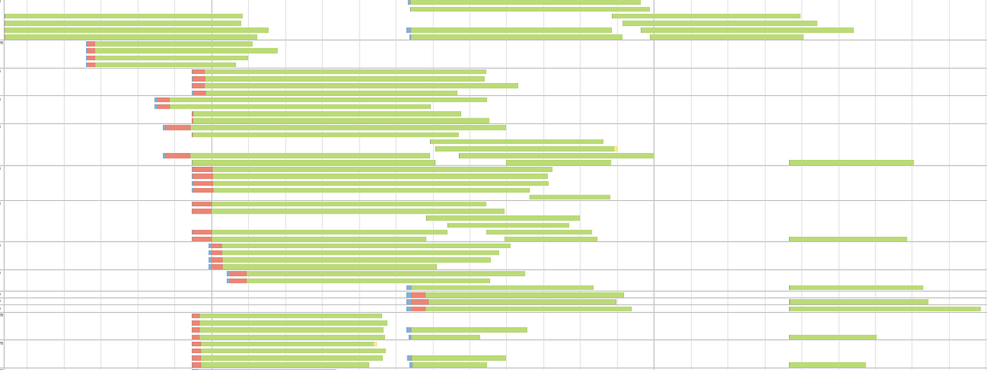
Very soon I realized that things are not that easy as I used to believe. And that same discovery is probably the reason why you landed on this article. For example, I would bet that you will find the following image quite familiar:
As you may already know the above is a typical manifestation of data skewness during a join operation: one task will take forever to complete just because all the effort of the join is put on a single executor process.
Oversimplifying how Spark joins tables
Looking at what tables we usually join with Spark, we can identify two situations: we may be joining a big table with a small table or, instead, a big table with another big table. Of course, during Spark development we face all the shades of grey that are between these two extremes!
Sticking to use cases mentioned above, Spark will perform (or be forced by us to perform) joins in two different ways: either using Sort Merge Joins if we are joining two big tables, or Broadcast Joins if at least one of the datasets involved is small enough to be stored in the memory of the single all executors. Note that there are other types of joins (e.g. Shuffle Hash Joins), but those mentioned earlier are the most common, in particular from Spark 2.3.
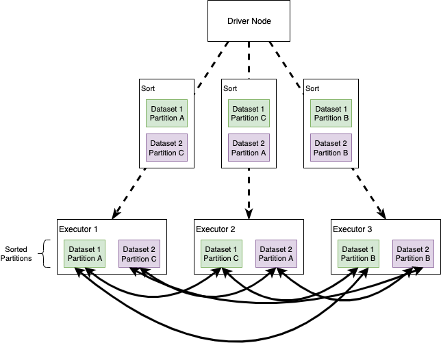
Sort Merge Joins
When Spark translates an operation in the execution plan as a Sort Merge Join it enables an all-to-all communication strategy among the nodes: the Driver Node will orchestrate the Executors, each of which will hold a particular set of joining keys. Before running the actual operation, the partitions are first sorted (this operation is obviously heavy itself). As you can imagine this kind of strategy can be expensive: nodes need to use the network to share data; note that Sort Merge Joins tend to minimize data movements in the cluster, especially compared to Shuffle Hash Joins.
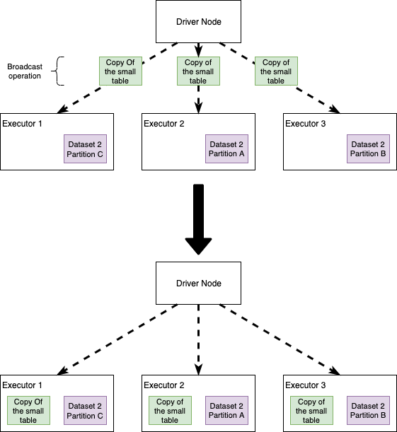
Broadcast Joins
Broadcast joins happen when Spark decides to send a copy of a table to all the executor nodes. The intuition here is that, if we broadcast one of the datasets, Spark no longer needs an all-to-all communication strategy and each Executor will be self-sufficient in joining the big dataset records in each node, with the small (broadcasted) table. We'll see that this simple idea improves performance… usually.
Wrapping up our enemies
Some of the biggest villains that we may face during join operations are:
- Data Skewness: the key on which we are performing the join is not evenly distributed across the cluster, causing one of the partitions to be very large and not allowing Spark to execute operations in parallel and/or congesting the network. Note that Skewness is a problem that affects many parallel computation systems: the keyword here is "parallel", we can take advantage of these tools only if we are able to execute multiple operations at the same time, so any data processing system that finds itself in some kind of skewed operation will suffer from similar problems (e.g. it also happens running Branch-and-Bound algorithms for Mixed-Integer Linear Programming Optimization).
- All-to-all communication strategy
- Limited executors memory
An important note before delving into some ideas to optimize joins: sometimes I will use the execution times to compare different join strategies. Actually, a lower absolute execution time does not imply that one method is absolutely better than the other. Performance also depends on the Spark session configuration, the load on the cluster and the synergies among configuration and actual code. So, read what follows with the intent of gathering some ideas that you'll probably need to tailor on your specific case!
Broadcasting or not broadcasting
First of all, let's see what happens if we decide to broadcast a table during a join. Note that the Spark execution plan could be automatically translated into a broadcast (without us forcing it), although this can vary depending on the Spark version and on how it is configured.
We will be joining two tables: fact_table and dimension_table. First of all, let's see how big they are:
          fact_table.count // #rows 3,301,889,672
dimension_table.count // #rows 3,922,556
In this case, the data are not skewed and the partitioning is all right — you'll have to trust my word. Note that the dimension_table is not exactly "small" (although size is not information that we can infer by only observing the number of rows, we'd rather prefer to look at the file size on HDFS).
By the way, let's try to join the tables without broadcasting to see how long it takes:
Output: Elapsed time: 215.115751969s Now, what happens if we broadcast the dimension table? By a simple addition to the join operation, i.e. replace the variable dimension_table with broadcast(dimension_table), we can force Spark to handle our tables using a broadcast:
Output: Elapsed time: 61.135962017s The broadcast made the code run 71% faster! Again, read this outcome having in mind what I wrote earlier about absolute execution time.
Is broadcasting always good for performance? Not at all! If you try to execute the snippets above giving more resources to the cluster (in particular more executors), the non-broadcast version will run faster than the broadcast one! One reason why this happens is because the broadcasting operation is itself quite expensive (it means that all the nodes need to receive a copy of the table), so it's not surprising that if we increase the amount of executors that need to receive the table, we increase the broadcasting cost, which suddenly may become higher than the join cost itself.
It's important to remember that when we broadcast, we are hitting on the memory available on each Executor node (here's a brief article about Spark memory). This can easily lead to Out Of Memory exceptions or make your code unstable: imagine to broadcast a medium-sized table. You run the code, everything is fine and super fast. A couple of months later you suddenly find out that your code breaks, OOM. After some hours of debugging, you may discover that the medium-sized table you broadcast to make your code fast is not that "medium" anymore. Takeaway, if you broadcast a medium-sized table, you need to be sure it will remain medium-sized in the future!
Skew it! This is taking forever!
Skewness is a common issue when you want to join two tables. We say a join is skewed when the join key is not uniformly distributed in the dataset. During a skewed join, Spark cannot perform operations in parallel, since the join's load will be distributed unevenly across the Executors.
Let's take our old fact_table and a new dimension:
          fact_table.count // #rows 3,301,889,672
dimension_table2.count // #rows 52
Great our dimension_table2 is very small and we can decide to broadcast it straightforward! Let's join and see what happens:
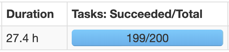
Output: Elapsed time: 329.991336182s Now, observe on the SparkUI what happened to the tasks during the execution:
As you can see in the image above, one of the tasks took much more time to complete compared to the others. This is clearly an indication of skewness in the data — and this conjecture would be easily verifiable by looking at the distribution of the join key in the fact_table.
To make things work, we need to find a way to redistribute the workload to improve our join's performance. I want to propose two ideas:
- Option 1: we can try to repartition our fact table, in order to distribute the effort in the nodes
- Option 2: we can artificially create a repartitioning key (key salting)
Option 1: Repartition the table
We can select a column that is uniformly distributed and repartition our table accordingly; if we combine this with broadcasting, we should have achieved the goal of redistributing the workload:
Output: Elapsed time: 106.708180448s Note that we want to choose a column also looking at the cardinality (e.g. I wouldn't choose a key with "too high" or "too low" cardinality, I let you quantify those terms).
Important note: if you cannot broadcast the dimension table and you still want to use this strategy, the left side and the right side of the join need to be repartitioned using the same partitioner! Let's see what happens if we don't.
Consider the following snippet and let's look at the DAG on the Spark UI
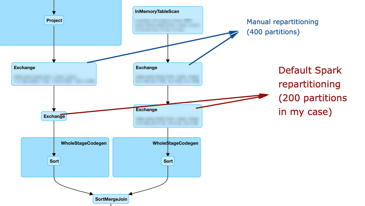
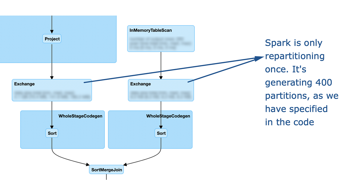
As you can see, it this case my repartitioning is basically ignored: after it is performed, spark still decides to re-exchange the data using the default configuration. Let's look at how the DAG changes if we use the same partitioner:
Option 2: Key salting
Another strategy is to forge a new join key!
We still want to force spark to do a uniform repartitioning of the big table; in this case, we can also combine Key salting with broadcasting, since the dimension table is very small.
The join key of the left table is stored into the field dimension_2_key, which is not evenly distributed. The first step is to make this field more "uniform". An easy way to do that is to randomly append a number between 0 and N to the join key, e.g.:
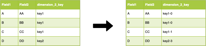
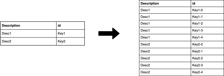
As you can see we modified the dimension_2_key which is now "uniformly" distributed, we are on the right path to a better workload on the cluster. We have modified the join key, so we need to do the same operation on the dimension table. To do so, we create for each "new" key value in the fact table, a corresponding value in the dimension: for each value of the id in the dimension table we generate N values in which we append to the old ids the numbers in the [0,N] interval. Let's make this clearer with the following image:
At this point, we can join the two datasets using the "new" salted key.
This simple trick will improve the degree of parallelism of the DAG execution. Of course, we have increased the number of rows of the dimension table (in the example N=4). A higher N (e.g. 100 or 1000) will result in a more uniform distribution of the key in the fact, but in a higher number of rows for the dimension table!
Let's code this idea.
First, we need to append the salt to the keys in the fact table. This is a surprisingly challenging task, or, better, it's a decision point:
- We can use a UDF: easy, but can be slow because Catalyst is not very happy with UDFs!
- We can use the "rand" SQL operator
- We can use the monotonically_increasing_id function
Just for fun, let's go with this third option (it also appear to be a bit faster)
Now we need to "explode" the dimension table with the new key. The fastest way that I have found to do so is to create a dummy dataset containing the numbers between 0 and N (in the example between 0 and 1000) and cross-join the dimension table with this "dummy" dataset:
Finally, we can join the tables using the salted key and see what happens!
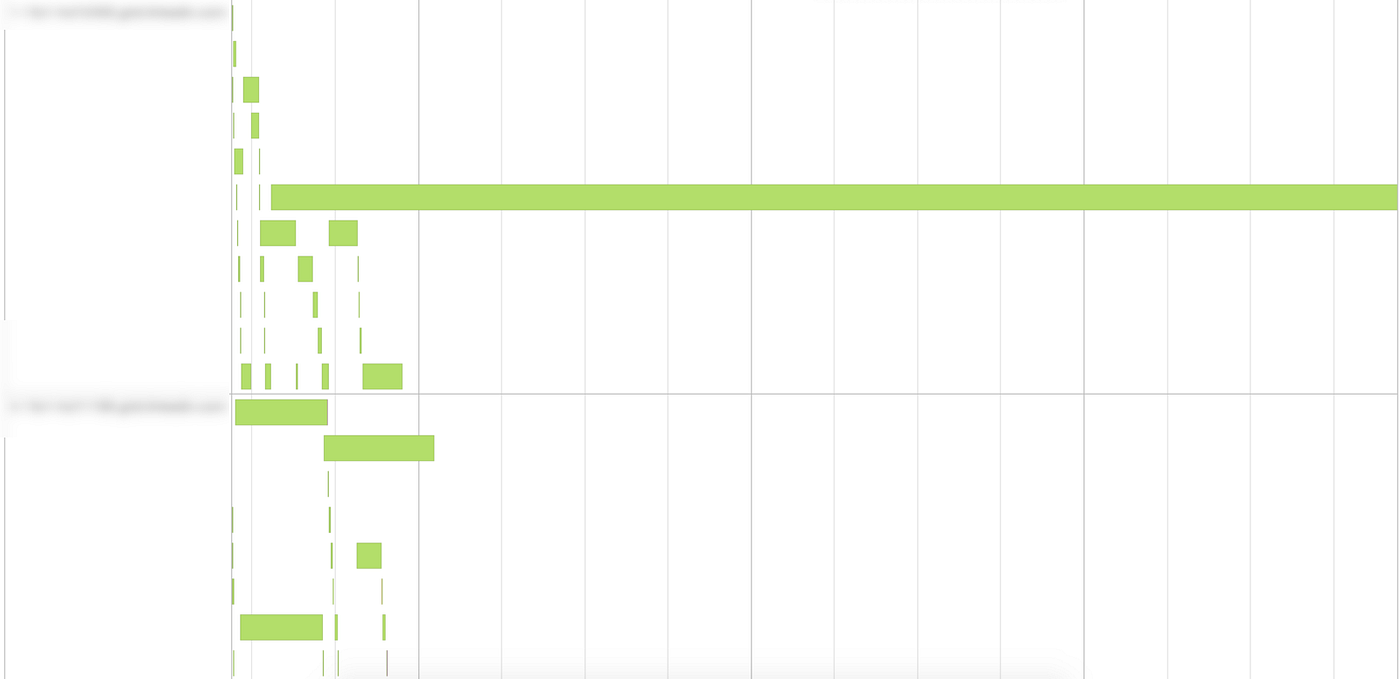
Output: Elapsed time: 182.160146932s Again, execution time is not really a good indicator to understand our improvement, so let's look at the event timeline:
As you can see we greatly increased the parallelism.
In this case, a simple repartitioning plus broadcast, worked better than crafting a new key. Note that this difference is not due to the join, but to the random number generation during the fact table lift.
Takeaways
- Joins can be difficult to tune since performance are bound to both the code and the Spark configuration (number of executors, memory, etc.)
- Some of the most common issues with joins are all-to-all communication between the nodes and data skewness
- We can avoid all-to-all communication using broadcasting of small tables or of medium-sized tables if we have enough memory in the cluster
- Broadcasting is not always beneficial to performance: we need to have an eye for the Spark config
- Broadcasting can make the code unstable if broadcast tables grow through time
- Skewness leads to an uneven workload on the cluster, resulting in a very small subset of tasks to take much longer than the average
- There are multiple ways to fight skewness, one is repartitioning.
- We can create our own repartitioning key, e.g. using the key salting technique
Check out these other articles!
Source: https://towardsdatascience.com/the-art-of-joining-in-spark-dcbd33d693c
0 Response to "Spark Easy to Write Many Join Query"
Post a Comment